Parameter selection with CroptimizR

Samuel Buis

2026-02-10

Introduction

This vignette illustrates a general workflow for parameter estimation and selection in crop models using CroptimizR and CroPlotR.
The workflow presented here implements the parameter selection algorithm described in Wallach et al. (2023), which provides a detailed methodology for stepwise parameter estimation.

This parameter estimation and selection algorithm proceeds through a sequence of successive steps. Its core idea is to distinguish between major parameters, which are systematically estimated in order to reduce bias, and candidate parameters, whose estimation is optional.

Major parameters are chosen for their strong and consistent influence on model outputs across all environments. A good candidate for this category typically affects simulated values in all environments.

Candidate parameters are those expected to explain part of the remaining variability between environments, but for which it is not always clear whether estimating them will improve model performance.

In the algorithm, major parameters are estimated first using an Ordinary Least Square (OLS) criterion. Candidate parameters are then added one by one to the set of estimated parameters and retained only if they lead to an improvement in an information criterion value (e.g., Akaike or Bayesian Information Criterion). Candidate parameters that are not selected are kept fixed at their default values.

Candidate parameters should be ordered, as far as possible, according to decreasing expected importance. While there is no strict limit on the number of candidate parameters, increasing this number directly increases the computational cost of the procedure.

Using an information criterion helps the algorithm limit overfitting, because it is calculated as the sum of a term measuring the fit of simulated values to observations and a penalty that increases with the number of estimated parameters.

Study Case

The crop model input data used in this example comes from a maize crop experiment (see description in Wallach et al., 2011). To illustrate the calibration procedure, julian days of two phenological stages were simulated from this dataset on 8 different environments (called situations in CroptimizR language) and then used as observations, after adding some random errors.

The STICS crop model is used in this example. Initialization steps required by the use of this model (definition of the model_options argument of the estim_param function) are hidden in this example for sake of brevity. They are detailed in the vignette Parameter estimation with CroptimizR: a simple case using the STICS crop Model.

Note however that CroptimizR can be applied to any crop model, provided that a suitable wrapper is available. Guidelines and examples for implementing wrappers are provided in the Designing a model wrapper vignette.

Wrappers already exist for several models. For more details, see the Get started page or contact the authors.

Plotting the observations

The observations are provided here in the obs_list object, in the format required by CroptimizR, i.e. as a named list of data frames (or tibble), each element being named after the corresponding situation (see the Get started vignette of CroptimizR for details).

In this example, the variables corresponding to the two observed stages considered are called iamfs and ilaxs. They correspond to the julian days (from the beginning of the sowing year) of “end juvenile” and “maximum LAI” stages as defined in the STICS crop model.

# Show the observations for the first two situations
obs_list[1:2]

## $`bo96iN+`
##         Date iamfs ilaxs
## 1 1996-10-15   168   230
## 
## $bou00t1
##         Date iamfs ilaxs
## 1 2000-11-01   181   221

The 8 situations are called here bo96iN+, bou00t1, bou00t3, bou99t1, bou99t3, lu96iN+, lu96iN6 and lu97iN+.

Let’s plot the values of these observations:

obs_df <- dplyr::bind_rows(obs_list) %>% tidyr::pivot_longer(
  cols = c("iamfs", "ilaxs"), names_to = "stage"
)
ggplot(obs_df, aes(x = stage, y = value)) +
  geom_boxplot()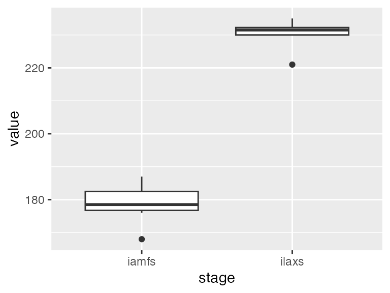

The “end juvenile” stage occurred around day 180 after sowing, while the “maximum LAI” stage occurred around day 230 after sowing.

Setting information on the parameters to estimate

The whole list of parameters to estimate and their lower and upper bounds (noted resp. lb and ub) must be provided in the param_info argument of the estim_param function.

In this example, we will consider 5 parameters of the STICS crop model: stlevamf, stamflax, tdmin, stressdev and tdmax.

param_info <- list(
  lb = c(stlevamf = 100, stamflax = 300, tdmin = 4, stressdev = 0, tdmax = 25),
  ub = c(stlevamf = 500, stamflax = 800, tdmin = 8, stressdev = 1, tdmax = 32)
)

Lower or upper bounds can be set to -Inf or Inf, respectively. In such cases, initial values must be provided for the corresponding parameters (see ?estim_param for further details).

Candidate parameters must be specified through the candidate_param argument of the estim_param function. This vector must be ordered from those thought to be the most influential on the considered variable, to the least influential. This ordering is important, as it directly determines the sequence in which candidate parameters are considered and tested during the stepwise parameter selection procedure.

In this example, 3 parameters were considered as candidates.

candidate_param <- c("tdmin", "stressdev", "tdmax")

Parameters that are included in param_info but not listed in candidate_param are treated as major parameters and are therefore systematically estimated at all steps of the procedure. In this example, stlevamf and stamflax belong to this category and are estimated regardless of the selected candidate parameters.

Choosing the default parameters values

Default values for the non-estimated parameters and for the candidate parameters can be defined in the forced_param_values argument of the estim_param function.

forced_param_values <- c(tdmin = 5.0, stressdev = 0.2, tdmax = 30.0)

These values will be used at each step for which these parameters are not estimated.

Setting optimization options

During the first step of the algorithm, all major parameters are estimated simultaneously, starting from randomly selected initial values. For subsequent steps, the initial values of parameters that have already been estimated are fixed at their previously estimated values, and only the initial value of the newly added candidate parameter is randomly drawn. As a consequence, Wallach et al. (2023) recommend performing a larger number of optimization repetitions for the first step (typically 10), and fewer repetitions for the subsequent steps (typically 5). This strategy is implemented as follows:

optim_options <- list(nb_rep = c(10, 5))

Running the optimization

A single call to the estim_param function is sufficient to run the complete parameter estimation and selection procedure.

Compared with the simple example presented in https://SticsRPacks.github.io/CroptimizR/articles/Parameter_estimation_simple_case.html , it is important here to explicitly define the crit_function argument. The stepwise parameter selection procedure illustrated in this vignette is currently implemented for an Ordinary Least Squares objective function, provided by crit_ols, which is not the default criterion used by estim_param.

Note also the use of the forced_param_values and candidate_param arguments, which respectively control the values of non-estimated parameters and the sequential inclusion of candidate parameters during the selection process.

By default, estim_param uses the corrected Akaike Information Criterion (AICc) for parameter selection. In this example, the Bayesian Information Criterion (BIC) is used instead, as specified through the info_crit_func argument.

res <- estim_param(
  obs_list = obs_list,
  model_function = model_wrapper,
  model_options = model_options,
  crit_function = crit_ols,
  optim_options = optim_options,
  param_info = param_info,
  forced_param_values = forced_param_values,
  candidate_param = candidate_param,
  info_crit_func = list(CroptimizR::BIC),
  out_dir = data_dir
)

At the end of the execution, some information such as the selected step number, the list of selected parameters, their estimated values and some stats about the execution time are printed in the R console:

...
# -- Summary of the Parameter Selection procedure results
#
# Selected step: 2
# Selected parameters: stlevamf,stamflax,tdmin
# Estimated value for stlevamf :  321.18
# Estimated value for stamflax :  589.73
# Estimated value for tdmin :  7.96
#
# A table summarizing the results obtained at the different steps  is stored in  C:/Users/sbuis/AppData/Local/Temp/RtmpwRzZkP/data-master/study_case_1/V9.0/param_selection_steps.csv
# Graphs and detailed results obtained for the different steps can be  found in  C:/Users/sbuis/AppData/Local/Temp/RtmpwRzZkP/data-master/study_case_1/V9.0/param_select_step# folders.
#
# Average time for the model to simulate all required situations: 4.1 sec elapsed
# Total number of criterion evaluation: 806
# Total time of model simulations: 3293 sec elapsed
# Total time of parameter estimation process: 3314 sec elapsed
# ----------------------

In this case, the object returned by the estim_param function contains the results corresponding to the selected step, as well as a data frame named param_selection_steps that provides detailed information for all steps of the parameter selection procedure. For each minimization step, param_selection_steps reports the set of estimated parameters, their initial and final values, and the associated values of the sum of squares and information criteria. The selected step is identified in the last column of this data frame. For convenience, the same information is also written to a CSV file (param_selection_steps.csv), saved either in the current working directory or in the directory specified by the out_dir argument of estim_param.

df <- read.csv("ResultsParameterSelection/param_selection_steps.csv", sep = ";")
knitr::kable(df)

Estimated.parameters	Initial.parameter.values	Final.values	Initial.Sum.of.squared.errors	Final.Sum.of.squared.errors	BIC	Selected.step
stlevamf, stamflax	356.22, 522.43	404.58, 739.23	2960	147	41.03
stlevamf, stamflax, tdmin	404.58, 739.23, 7.67	321.18, 589.73, 7.96	4242	91	36.13	X
stlevamf , stamflax , tdmin , stressdev	321.18, 589.73, 7.96, 1.00	321.18, 589.73, 7.96, 1.00	91	91	38.90
stlevamf, stamflax, tdmin , tdmax	321.18, 589.73, 7.96, 30.20	321.18, 589.73, 7.96, 31.07	91	91	38.90

In this example, the selected parameter set consists of stlevamf, stamflax, and tdmin, corresponding to the lowest value of the BIC among all tested steps.

The complete object returned by the estim_param function is also saved to disk in the file optim_results.Rdata.

Standard result files and diagnostic plots produced by estim_param for each step of the procedure are stored in the param_select_step# folders.

Generating diagnostics using CroPlotR

To generate diagnostic plots, the model wrapper is first run using the estimated values of the selected parameters, while all remaining parameters are set to their default values. These values are passed to the model through the param_values argument.

param_values <- c(res$final_values, res$forced_param_values)
sim_after_optim <- model_wrapper(
  param_values = param_values,
  model_options = model_options,
  var = c("iamfs", "ilaxs")
)

Once the simulations have been performed, simulated and observed values can be compared graphically using the plotting functions provided by CroPlotR.

In particular, scatter plots of simulated versus observed values can be produced as follows:

plot(sim_after_optim$sim_list, obs = obs_list, type = "scatter")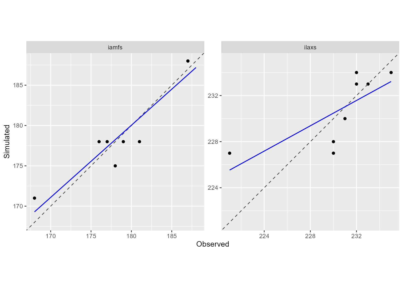

In addition to graphical diagnostics, quantitative performance metrics can be computed for each variable. In this example, the Mean Squared Error (MSE) and its decomposition are calculated using the summary function from CroPlotR.

summary(sim_after_optim$sim_list,
  obs = obs_list,
  stats = c("MSE", "Bias2", "SDSD", "LCS")
)

## # A tibble: 2 × 7
##   group     situation      variable   MSE  Bias2   SDSD   LCS
##   <chr>     <chr>          <chr>    <dbl>  <dbl>  <dbl> <dbl>
## 1 Version_1 all_situations iamfs     4.38 0.0156 0.0637  4.92
## 2 Version_1 all_situations ilaxs     7    0.0625 1.14    6.78