Parameter estimation with CroptimizR: a simple case using the ApsimX crop Model
Patrice Lecharpentier
INRAE AgroclimSamuel Buis
INRAE EMMAHDrew Holzworth
2026-02-10
Source:vignettes/ApsimX_parameter_estimation_simple_case.Rmd
ApsimX_parameter_estimation_simple_case.RmdIntroduction
This document presents a simple example of parameter estimation using CroptimizR on a complex crop model.
For more advanced use cases, the following vignettes are available:
-
Simultaneous
estimation of specific and varietal plant parameters using a
multi-varietal dataset.
-
Parameter
selection procedure illustrating how to choose which parameters to
estimate.
-
AgMIP
Calibration Protocol demonstrating the application of the AgMIP
calibration workflow.
- Bayesian parameter estimation using the DREAM-zs algorithm.
Study Case
This example uses the ApsimX crop model. However, CroptimizR can be applied to any crop model, provided that a suitable wrapper is available. Guidelines and examples for implementing wrappers are provided in the Designing a model wrapper vignette.
Note that a similar example using the STICS crop model is available in another vignette.
Wrappers already exist for several models. For more details, see the Get started page or contact the authors.
The dataset used in this example comes from a maize crop experiment (see Wallach et al., 2011). It involves a single environment, a single observed variable, and two estimated parameters, just to illustrate how to use the package.
Parameter estimation is performed here using the Nelder-Mead simplex
method implemented in the R package nloptr.
Initialisation step
# Install and load the needed libraries
if (!require("CroptimizR")) {
  devtools::install_github("SticsRPacks/CroptimizR@*release")
  library("CroptimizR")
}
if (!require("CroPlotR")) {
  devtools::install_github("SticsRPacks/CroPlotR@*release")
  library("CroPlotR")
}
if (!require("ApsimOnR")) {
  devtools::install_github("hol430/ApsimOnR")
  library("ApsimOnR")
}
if (!require("dplyr")) {
  install.packages("dplyr", repos = "http://cran.irsn.fr")
  library("dplyr")
}
if (!require("ggplot2")) {
  install.packages("ggplot2", repos = "http://cran.irsn.fr")
  library("ggplot2")
}
if (!require("gridExtra")) {
  install.packages("gridExtra", repos = "http://cran.irsn.fr")
  library("gridExtra")
}

if (!require("tidyr")) {
  install.packages("tidyr", repos = "http://cran.irsn.fr")
  library(tidyr)
}

# DEFINE THE PATH TO THE LOCALLY INSTALLED VERSION OF APSIM (should be something
# like C:/path/to/apsimx/bin/Models.exe on windows, and /usr/local/bin/Models
# on linux)
apsimx_path <- "D:\\Home\\sbuis\\Documents\\OUTILS-INFORMATIQUE\\APSIM2025.04.7734.0\\bin\\Models.exe"
Set the list of situations and variables to consider in this example
sit_name <- "GattonRowSpacingRowSpace25cm"
# among "GattonRowSpacingRowSpace25cm",
# "GattonRowSpacingRowSpace50cm",
# "GattonRowSpacingRowSpaceN0"

var_name <- c("Wheat.Leaf.LAI") # or "Wheat.AboveGround.Wt"
Run the model before optimization for a prior evaluation
In this case, the argument param_values of the wrapper
is not set: the values of the model input parameters are all read in the
model input files.
# Set the model options (see '? apsimx_wrapper_options' for details)
files_path <- system.file(file.path("extdata", "apsimx_files"),
  package = "ApsimOnR"
)
apsimx_file <- file.path(files_path, "template.apsimx")

# Setting met files path
met_files_path <- files_path

# Setting observed data files path
obs_files_path <- files_path

# Setting sqlite db tables names
predicted_table_name <- "DailyReport"
observed_table_name <- "Observed"

model_options <- apsimx_wrapper_options(
  apsimx_path = apsimx_path,
  apsimx_file = apsimx_file,
  variable_names = var_name,
  predicted_table_name = predicted_table_name,
  met_files_path = met_files_path,
  observed_table_name = observed_table_name,
  obs_files_path = obs_files_path
)

# Run the model (on all situations found in the apsimx_file)
sim_before_optim <- apsimx_wrapper(model_options = model_options)
Read and select the corresponding observations
We only keep observations for situation sit_name and
variable var_name (obs_list defines the list
of situations and variables that will be used in the parameter
estimation process).
# At the moment, observed data are read from the db file after the first
# simulation ran before optimization. But they may be loaded using the original
# xlsx data file (from the files_path)

obs_list <- read_apsimx_output(
  sim_before_optim$db_file_name,
  model_options$observed_table_name,
  model_options$variable_names,
  names(sim_before_optim$sim_list)
)
obs_list <- filter_obs(obs_list, situation = sit_name, include = TRUE)
Set information on the parameters to estimate
param_info must contain information about the
parameters that will be estimated in the parameter estimation process
from the situations, variables and dates defined in
obs_list.
It must include the definition of their upper and lower bounds (-Inf and Inf can be used). This will determine the list of estimated parameters.
Initial values for the minimization can also be provided in
param_info (see ? estim_param).
# 2 parameters here: ExtinctionCoeff and RUE, of bounds [0.4,0.6] and [1.4,1.6]
param_info <-
  list(
    lb = c(
      .Simulations.Replacements.Wheat.Leaf.ExtinctionCoeff.VegetativePhase.FixedValue = 0.4,
      .Simulations.Replacements.Wheat.Leaf.Photosynthesis.RUE.FixedValue = 1.4
    ),
    ub = c(
      .Simulations.Replacements.Wheat.Leaf.ExtinctionCoeff.VegetativePhase.FixedValue = 0.6,
      .Simulations.Replacements.Wheat.Leaf.Photosynthesis.RUE.FixedValue = 1.6
    )
  )
Set options for the parameter estimation method
optim_options should contain the options of the
parameter estimation method. Here we defined a few options for the
simplex method of the nloptr package (default method in
estim_param). The full set of options for the simplex method can be
found in the vignette
of nloptr package.
The number of repetitions nb_rep is advised to be set at
least to 5, while 10 is a reasonable maximum value. maxeval
should be used to stop the minimization only if results have to be
produced within a given duration, otherwise set it to a high value so
that the minimization stops when the criterion based on the relative
tolerance xtol_rel is satisfied.
optim_options <- list()
optim_options$nb_rep <- 7 # Number of repetitions of the minimization
# (each time starting with different initial
# values for the estimated parameters)
optim_options$maxeval <- 500 # Maximum number of evaluations of the
# minimized criteria
optim_options$xtol_rel <- 1e-03 # Tolerance criterion between two iterations
# (threshold for the relative difference of
# parameter values between the 2 previous
# iterations)

optim_options$ranseed <- 1234 # set random seed so that each execution give the
#  same results. If you want randomization,
# don't set it.
Run the optimization
The Nelder-Mead simplex is the default method => no need to set
the optim_method argument if you want to use it. The list of available
methods is detailed here.
Same for crit_function: a value is set by default
(crit_log_cwss, see ? crit_log_cwss or here
for more details and list of available criteria). Others will be
proposed in next versions of CroptimizR. The user can implement and give
in argument its own criterion (see inputs and outputs required in the
crit_log_cwss function).
res <- estim_param(
  obs_list = obs_list,
  model_function = apsimx_wrapper,
  model_options = model_options,
  optim_options = optim_options,
  param_info = param_info
)
The estimated values of the parameters are the following:
res$final_values## .Simulations.Replacements.Wheat.Leaf.ExtinctionCoeff.VegetativePhase.FixedValue
## 0.4321273
## .Simulations.Replacements.Wheat.Leaf.Photosynthesis.RUE.FixedValue
## 1.6000000Complementary graphs and data are stored in the folder which path is
given in the out_dir argument of estim_param
(equal to getwd() by default). Among them, the
EstimatedVSinit.pdf file contains the following
figures:
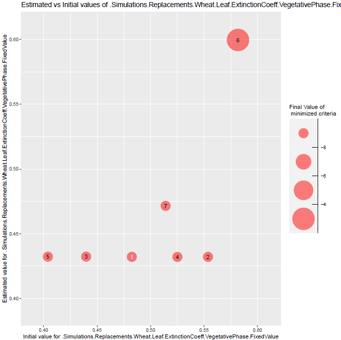

Figure 1: plots of estimated vs initial values of parameters ExtinctionCoeff and RUE. Numbers represent the repetition number of the minimization and the size of the bubbles the final value of the minimized criterion. The number in white, 2 in this case, is the minimization that lead to the minimal value of the criterion among all repetitions. In this case, minimizations converge towards different values for the parameters (3 for ExtinctionCoeff and 2 for RUE), which indicates the presence of local minima. Values of RUE are very close to the upper bound value. In realistic calibration cases this may indicate the presence of a large error in the observation values or in the simulated output values (this simple case with only one situation does not allow to derive such conclusion).
Run the model after optimization
In this case, the param_values argument is set so that
estimated values of the parameters overwrite the values defined in the
model input file (’.apsimx`).
sim_after_optim <- apsimx_wrapper(
  param_values = res$final_values,
  model_options = model_options
)
Plot the results
Here we use the CroPlotR package for comparing simulations and observations. As CroptimizR, CroPlotR can be used with any crop model.
p <- plot(sim_before_optim$sim_list, obs = obs_list, select_dyn = c("common"))
p1 <- p[[sit_name]] + labs(title = "Before Optimization")

p <- plot(sim_after_optim$sim_list, obs = obs_list, select_dyn = c("common"))
p2 <- p[[sit_name]] + labs(title = "After Optimization") +
  ylim(NA, ggplot_build(p1)$layout$panel_params[[1]]$y.range[2])

p <- grid.arrange(grobs = list(p1, p2), nrow = 1, ncol = 2)
# Save the graph
ggsave(
  paste0("sim_obs_plots", ".png"),
  plot = p
)
this gives:
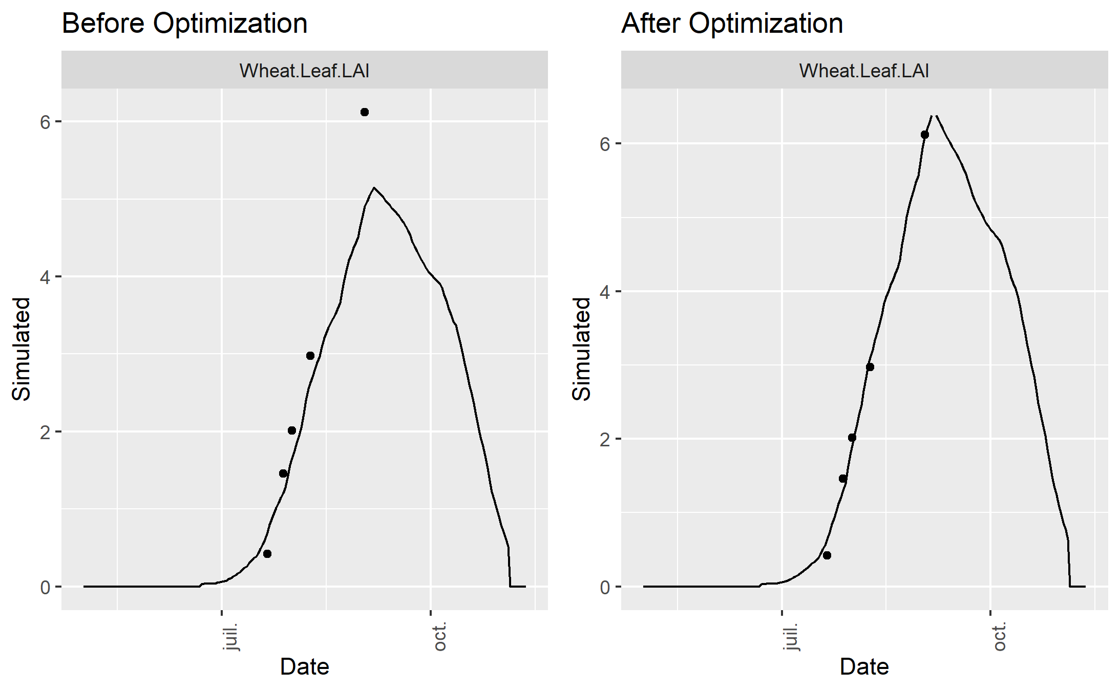
Figure 2: plots of simulated and observed target variable before and after optimization. The gap between simulated and observed values has been drastically reduced: the minimizer has done its job!