Parameter estimation with CroptimizR: a simple case using the STICS crop Model
Samuel Buis
2026-02-10
Source:vignettes/Parameter_estimation_simple_case.Rmd
Parameter_estimation_simple_case.RmdIntroduction
This document presents a simple example of parameter estimation using CroptimizR on a complex crop model.
For more advanced use cases, the following vignettes are
available:
- Simultaneous
estimation of specific and varietal plant parameters using a
multi-varietal dataset.
- Parameter
selection procedure illustrating how to choose which parameters to
estimate.
- AgMIP
Calibration Protocol demonstrating the application of the AgMIP
calibration workflow.
- Bayesian
parameter estimation using the DREAM-zs algorithm.
Study Case
This example uses the STICS crop model. However, CroptimizR can be applied to any crop model, provided that a suitable wrapper is available. Guidelines and examples for implementing wrappers are provided in the Designing a model wrapper vignette.
Note that a similar example using the ApsimX crop model is available in another vignette.
Wrappers already exist for several models. For more details, see the Get started page or contact the authors.
The dataset used in this example comes from a maize crop experiment (see Wallach et al., 2011). It involves a single environment, a single observed variable, and two estimated parameters, just to illustrate how to use the package.
Parameter estimation is performed here using the Nelder-Mead simplex
method implemented in the R package nloptr.
Initialisation step
# Install and load the needed libraries
if (!require("SticsRPacks")) {
  devtools::install_github("SticsRPacks/SticsRPacks")
  library("SticsRPacks")
}
# DEFINE THE PATH TO YOUR LOCALLY INSTALLED VERSION OF JAVASTICS
javastics_path <- path_to_JavaStics

# Download the example USMs and define the path to the JavaStics workspace
# (JavaStics XML input files):
data_dir <- file.path(
  SticsRFiles::download_data(
    example_dirs = "study_case_1",
    stics_version = "V9.0"
  )
)

javastics_workspace_path <- file.path(data_dir, "XmlFiles")
Generate Stics input files from JavaStics input files
The Stics wrapper function used in CroptimizR works on Stics input
files (text formatted files new_travail.usm, climat.txt, …) stored per
USMs in different directories (which names must be the USM names).
stics_inputs_path is here the path of the directory that
will contain these USMs folders.
If you start from xml formatted input files (JavaStics format:
usms.xml, sols.xml, …) the following lines allow generating txt files
from xml files. In this example, xml files are stored in
javastics_workspace_path and the Stics input files (test
format) will be stored in
stics_inputs_path=file.path(data_dir,"TxtFiles")
stics_inputs_path <- file.path(data_dir, "TxtFiles")
dir.create(stics_inputs_path, showWarnings = FALSE)

gen_usms_xml2txt(
  javastics = javastics_path,
  workspace = javastics_workspace_path,
  out_dir = stics_inputs_path,
  verbose = TRUE
)
Run the model before optimization for a prior evaluation
Here model parameters values are read in the model input files.
# Set the model options (see '? stics_wrapper_options' for details)
model_options <-
  stics_wrapper_options(
    javastics = javastics_path,
    workspace = stics_inputs_path,
    parallel = FALSE
  )

# Run the model on all situations found in stics_inputs_path
sim_before_optim <- stics_wrapper(model_options = model_options)
Read and select the observations for the parameter estimation
For Stics, observation files must for the moment have exactly the same names as the corresponding USMs and be stored in a unique folder to be read by the get_obs function. This will be improved in next versions.
In this example, we only keep observations for situation (i.e. USM
for Stics) sit_name and variable var_name.
obs_list defines the list of situations,
variables and dates that will be used to estimate the parameters. Use
the function filter_obs (see ? filter_obs) for
removing situations, variables and/or dates from an observation
list.
In variables and parameters names, “(*)” must be replaced by “_*” to be handled by R (e.g. lai(n) is denoted here lai_n).
sit_name <- "bo96iN+" # can be a vector of situation names if you want to
# consider several, e.g. c("bo96iN+","bou00t1")
var_name <- "lai_n" # can be a vector of variable names if you want to
# consider several, e.g. c("lai_n","masec_n")
obs_list <- get_obs(javastics_workspace_path, usm = sit_name)
obs_list <- filter_obs(obs_list, var = var_name, include = TRUE)
Set information on the parameters to estimate
param_info must contain information about the
parameters that will be estimated in the parameter estimation process
from the situations, variables and dates defined in
obs_list.
It must include the definition of their upper and lower bounds (-Inf and Inf can be used). This will determine the list of estimated parameters.
All the numerical parameters which values can be provided to the model through its R wrapper can be estimated using the provided parameter estimation methods (although it may not work well for integer parameters).
Initial values for the minimization can also be provided in
param_info (see ? estim_param).
Set options for the parameter estimation method
optim_options must contain the options of the parameter
estimation method. Here we defined a few important options for the
simplex method of the nloptr package (default method in estim_param). To
see the full set of options available for the simplex method, type
? nl.opts
The number of repetitions is advised to be set to at least 5, while
10 is a reasonable maximum value. maxeval should be used to
stop the minimization only if results have to be produced within a given
duration, otherwise set it to a high value so that the minimization
stops when the criterion based on xtol_rel is
satisfied.
optim_options <- list()
optim_options$nb_rep <- 7 # Number of repetitions of the minimization
# (each time starting with different initial
# values for the estimated parameters)
optim_options$maxeval <- 500 # Maximum number of evaluations of the
# minimized criteria
optim_options$xtol_rel <- 1e-03 # Tolerance criterion between two iterations
# (threshold for the relative difference of
# parameter values between the 2 previous
# iterations)
optim_options$ranseed <- 1234 # set random seed so that each execution give the
# same results
# If you want randomization, don't set it.
Run the optimization
The Nelder-Mead simplex is the default method => no need to set
the optim_method argument if you want to use it. The list of available
methods is detailed here.
Same for crit_function: a value is set by default
(crit_log_cwss, see ? crit_log_cwss or here
for more details and list of available criteria). Others will be
proposed in next versions of CroptimizR. The user can implement and give
in argument its own criterion (see inputs and outputs required in the
crit_log_cwss function).
res <- estim_param(
  obs_list = obs_list,
  model_function = stics_wrapper,
  model_options = model_options,
  optim_options = optim_options,
  param_info = param_info,
  out_dir = data_dir # path where to store the results
)
The estim_param function returns a list which is also
stored in the optim_results.Rdata file of the out_dir
folder.
This list contains different information depending on the method used. For the Nelder-Mead simplex method it includes among others:
- the final values estimated for the parameters
res$final_values## dlaimax durvieF
## 0.001614435 50.000000000- the initial and final values of the estimated parameters for each repetition of the minimization:
res$init_values## dlaimax durvieF
## 1 0.0010614022 101.05543
## 2 0.0016225903 228.02236
## 3 0.0019301103 343.82293
## 4 0.0011393688 365.02290
## 5 0.0007499945 278.11596
## 6 0.0023386301 156.76596
## 7 0.0018972162 95.83214
res$est_values## dlaimax durvieF
## [1,] 0.001604844 130.9555
## [2,] 0.001223672 382.3685
## [3,] 0.001224056 399.1707
## [4,] 0.001223849 362.6018
## [5,] 0.001223128 391.8069
## [6,] 0.001614435 50.0000
## [7,] 0.001223580 338.6791- the minimum value of the criterion among all repetitions and for all repetitions:
res$min_crit_value## [1] 4.915215
res$crit_values## [1] 5.146571 5.096751 5.096751 5.096751 5.096783 4.915215 5.096751the plots automatically generated (see their description here-after) in ggplot format (=> can be modified using standard ggplot commands)
elapsed time measurements (total time, total time of model simulations, average time of model simulations)
the list of values of the parameters and of the criterion for each evaluation during the minimization (
params_and_crit), ifinfo_level>=1the
nlovariable, a list returned by the nloptr function that contains detailed information on the results of the minimization for each repetition.
nlo is a list of size the number of repetitions. Each
element stores many information about the corresponding minimization,
including the number of iterations performed (field
iterations) and a message indicating why the minimization
stopped (field message).
Let’s print it for the repetition that leads to the minimum value of the criterion over all repetitions:
res$nlo[[res$ind_min_crit]]##
## Call:
## nloptr::nloptr(x0 = as.numeric(init_values[irep, ]), eval_f = main_crit,
## lb = bounds$lb, ub = bounds$ub, opts = list(algorithm = "NLOPT_LN_NELDERMEAD",
## xtol_rel = xtol_rel, maxeval = maxeval, ranseed = ranseed),
## crit_options = crit_options)
##
##
## Minimization using NLopt version 2.4.2
##
## NLopt solver status: 4 ( NLOPT_XTOL_REACHED: Optimization stopped because
## xtol_rel or xtol_abs (above) was reached. )
##
## Number of Iterations....: 55
## Termination conditions: xtol_rel: 0.001 maxeval: 500
## Number of inequality constraints: 0
## Number of equality constraints: 0
## Optimal value of objective function: 4.91521542817615
## Optimal value of controls: 0.001614435 50This data is also stored in the out_dir folder (file
optim_results.Rdata) along with a set of pdf files:
- the EstimatedVSinit.pdf file contains the following figures:
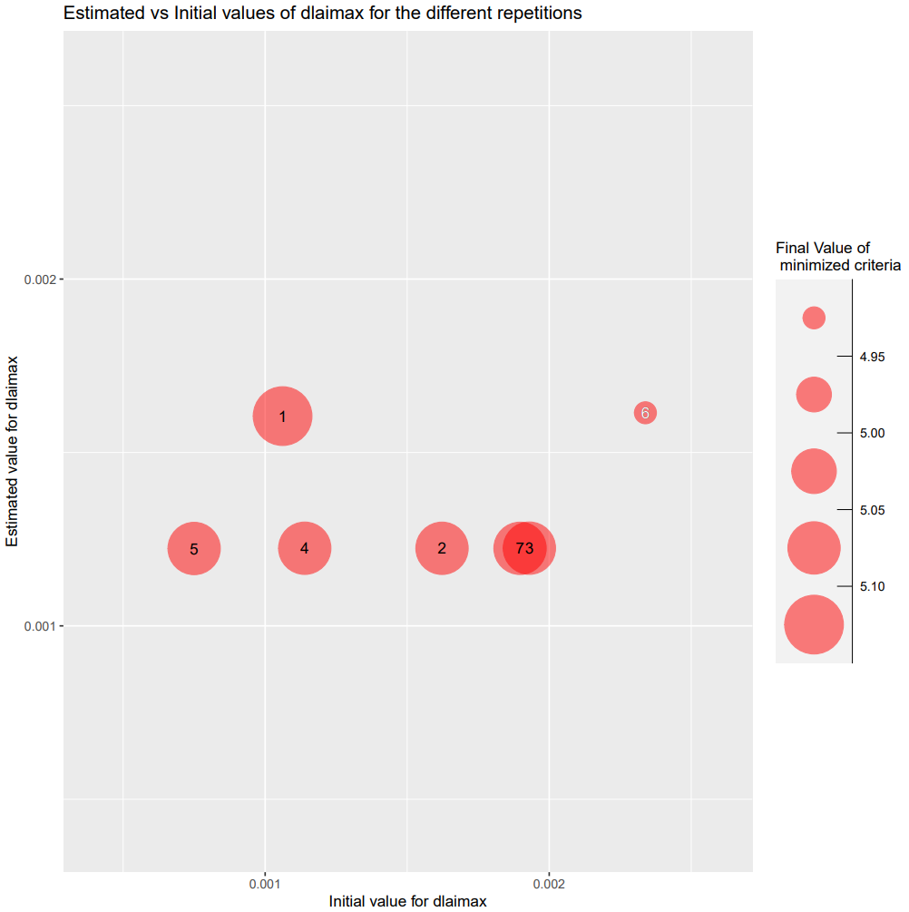

Figure 1: plots of estimated vs initial values of parameters dlaimax and durvieF. Numbers represent the repetition number of the minimization and the size of the bubbles the final value of the minimized criterion. The number in white, 6 in this case, is the minimization that leads to the minimal value of the criterion among all repetitions. In this case, the minimizations converge towards different values for the parameters, which indicates the presence of local minima. Values of durvieF are close to the bounds. In realistic calibration cases with many observed situations / variables / dates this may indicate the presence of biases in the observation values or in the model output values simulated (this simple case with only one situation does not allow to derive such conclusion).
- the ValuesVSit.pdf file contains:
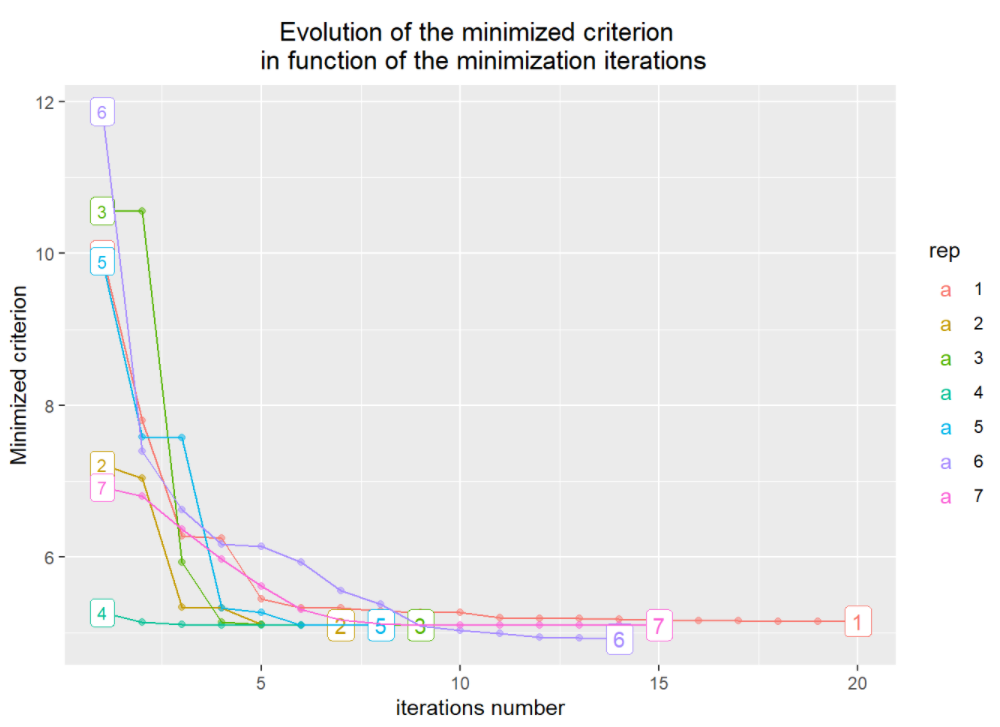


Figure 2: The top left figure displays the evolution of the minimized criterion value in function of the iterations of the minimization. Colors and labels represent the repetition number. The top right figure displays the evolution of the value of the dlaimax parameter in function of the iterations of the minimization. Labels represent the repetition number and colors the value of the minimized criterion. The figure at the bottom is the same but for the durvieF parameter.
- the ValuesVSit_2D.pdf file contains:
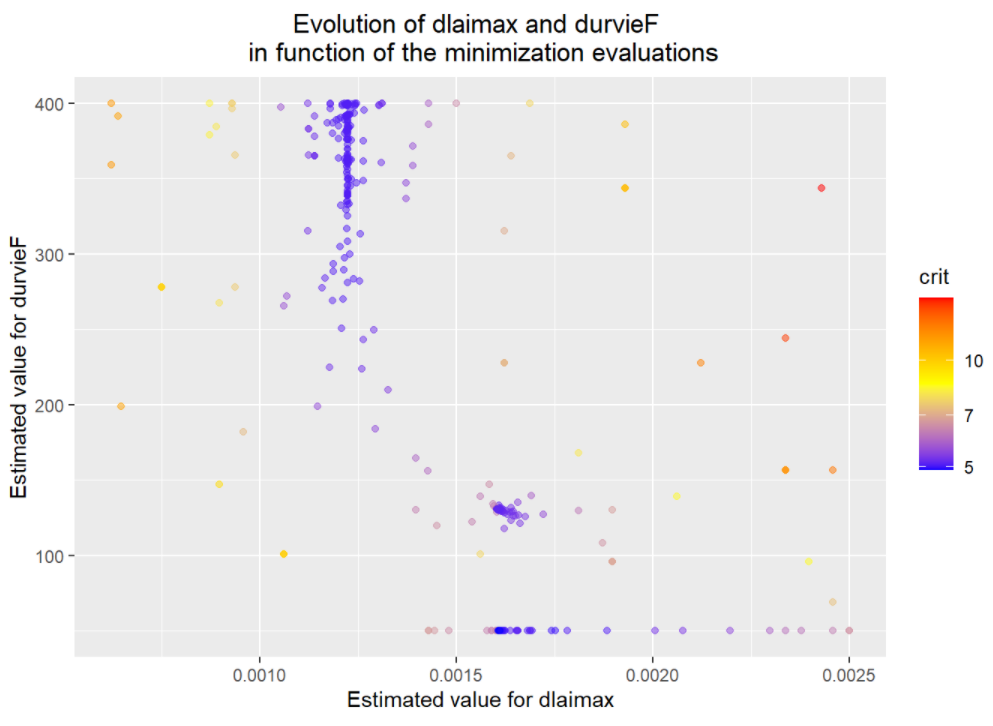
Figure 3: This figure displays all the values proposed by the minimizer for the durvieF (Y axis) and dlaimax (X-axis) parameters and the associated values of the minimized criterion (dot colors).
Run the model after optimization
We run here the Stics model using the estimated values of the
parameters. In this case, the param_values argument of the
stics_wrapper function is thus set so that estimated values of the
parameters overwrite the values defined in the model input files.
sim_after_optim <- stics_wrapper(
  param_values = res$final_values,
  model_options = model_options
)
Plot the results
Here we use the CroPlotR package for comparing simulations and observations. As CroptimizR, CroPlotR can be used with any crop model.
p <- plot(
  sim_before_optim$sim_list,
  obs = obs_list,
  select_dyn = c("common")
)

p1 <-
  p[[sit_name]] +
  labs(title = "Before Optimization") +
  theme(plot.title = element_text(size = 9, hjust = 0.5))

p <-
  plot(
    sim_after_optim$sim_list,
    obs = obs_list,
    select_dyn = c("common")
  )

p2 <- p[[sit_name]] +
  labs(title = "After Optimization") +
  ylim(
    NA,
    ggplot_build(p1)$layout$panel_params[[1]]$y.range[2]
  ) +
  theme(plot.title = element_text(size = 9, hjust = 0.5))

p <- grid.arrange(
  grobs = list(p1, p2),
  nrow = 1,
  ncol = 2,
  widths = c(5, 5)
)
# Save the graph
ggsave(
  file.path(
    data_dir,
    paste0("sim_obs_plots", ".png")
  ),
  plot = p
)
This gives:
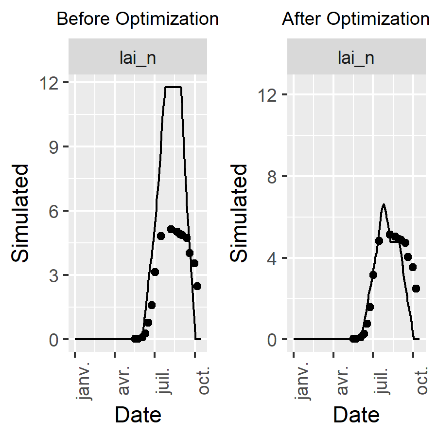
Figure 4: plots of simulated and observed target variable before and after optimization. The gap between simulated and observed values has been drastically reduced: the minimizer has done its job!