Estimating phenology following AgMIP-calibration phase III protocol

Introduction

This document presents how the AgMIP phase III protocol, designed to calibrate phenology of crop models, can be easily implemented using CroptimizR and CroPlotR packages.

This protocol is described in detail in Wallach et al (2022).

Its objective is to improve crop model parameters values using calibration for prediction of crop phenology.

Here is a brief description of its different steps:

Define the default values for all parameters that impact the simulation of phenology in the considered crop model.
Identify measured variables (phenological stages) to be fit within the dataset available.
Identify the nearly additive, obligatory parameters to be calibrated. The obligatory parameters are parameters that are nearly additive, i.e. such that changing the parameter has a similar effect for all environments (typically parameters that control degree days to the measured stages). Ideally, the number of almost additive parameters will be identical to the number of measured variables used. These parameters will be estimated at each stage of the parameter estimation process. Their estimation should lead to the elimination of bias between measured and estimated phenological stages.
Identify candidate parameters to be calibrated. The role of the candidate parameters is to reduce the variability between environments that remains after estimation of the obligatory parameters.
Calculate the optimal parameter values. A model selection algorithm is used to decide which parameters to estimate. First, all obligatory parameters are estimated. Then, each candidate parameter is added in turn to the list of estimated parameters, and only those that lead to a reduction of a model selection criterion (BIC) are retained for estimation. Otherwise, the parameter is kept at its default value. Each set of parameters are estimated by minimizing an Ordinary Least Square criterion (sum of squared differences between measured and simulated phenological stages considered on all the environments). The minimizations are performed using the Nelder-Mead simplex algorithm and repeated from multiple (randomly chosen or given) starting points. At the end, the parameters values resulting from the calibration process are the estimated and default values of the parameters that lead to the lowest value of the BIC criterion.

Study Case

The crop model input data used in this example comes from a maize crop experiment (see description in Wallach et al., 2011). To illustrate the calibration procedure, julian days of two phenological stages were simulated from this dataset on 8 different environments (called situations in CroptimizR language) and then used as observations, after adding some random errors.

The STICS crop model is used in this example. Initialization steps required by the use of this model (definition of the model_options argument of the estim_param function) are hidden in this example for sake of brevity. They are detailed in the vignette (https://SticsRPacks.github.io/CroptimizR/articles/Parameter_estimation_simple_case.html).

Plotting the observations

The observations are provided here in the obs_list object, in the format required by CroptimizR, i.e. a named list of data.frame.

In this example, the variables corresponding to the two observed stages considered are called “iamfs” and “ilaxs”. They correspond to the julian days (from the beginning of the sowing year) of “end juvenile” and “maximum LAI” stages as defined in the STICS crop model.

print(obs_list)

## $`bo96iN+`
##         Date iamfs ilaxs
## 1 1996-10-15   168   230
## 
## $bou00t1
##         Date iamfs ilaxs
## 1 2000-11-01   181   221
## 
## $bou00t3
##         Date iamfs ilaxs
## 1 2000-11-01   179   230
## 
## $bou99t1
##         Date iamfs ilaxs
## 1 1999-11-05   187   233
## 
## $bou99t3
##         Date iamfs ilaxs
## 1 1999-11-05   187   232
## 
## $`lu96iN+`
##         Date iamfs ilaxs
## 1 1996-10-16   177   232
## 
## $lu96iN6
##         Date iamfs ilaxs
## 1 1996-10-16   176   235
## 
## $`lu97iN+`
##         Date iamfs ilaxs
## 1 1997-10-10   178   231

The 8 situations are called here bo96iN+, bou00t1, bou00t3, bou99t1, bou99t3, lu96iN+, lu96iN6 and lu97iN+.

Let’s plot the values of these observations:

obs_df <- dplyr::bind_rows(obs_list) %>% tidyr::pivot_longer(
  cols = c("iamfs", "ilaxs"), names_to = "stage")
ggplot(obs_df, aes(x = stage, y = value)) + geom_boxplot()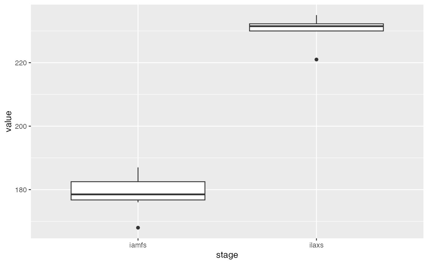

The “end juvenile” stage occurred around day 180 after sowing, while the “maximum LAI” stage occurred around day 230 after sowing.

Setting information on the parameters to estimate

The whole list of parameters to estimate and their lower and upper bounds (noted resp. lb and ub) must be provided in the param_info argument of the estim_param function.

In this example, we will consider 5 parameters of the STICS crop model: stlevamf, stamflax, tdmin, stressdev and tdmax.

param_info <- list(
  lb = c(stlevamf = 100, stamflax = 300, tdmin = 4, stressdev = 0, tdmax = 25),
  ub = c(stlevamf = 500, stamflax = 800, tdmin = 8, stressdev = 1, tdmax = 32)
  )

Note that -Inf or Ìnf can be used for, respectively, lower and upper bounds. In that case, initial values must be provided for the corresponding parameters (see ? estim_param for more details).

The list of candidate parameters must be provided in the candidate_param argument of
the estim_param function. Note that, as prescribed in the AgMIP protocol, this list must be ordered, from those thought to be the most important to those thought to be the least important.

In this example, 3 parameters were considered as candidates.

candidate_param <- c("tdmin", "stressdev", "tdmax")

The parameters not included in candidate_param but included in param_info will be considered as the nearly additive parameters, as defined in the protocol. In this example, stlevamf and stamflax are thus the nearly additive parameters that will be estimated at any step.

Choosing the default parameters values

Default values for the non-estimated parameters and for the candidate parameters can be defined in the forced_param_values argument of the estim_param function.

forced_param_values <- c(tdmin = 5.0, stressdev = 0.2, tdmax = 30.0)

These values will be used at each step for which these parameters are not estimated.

Setting optimization options

Following the AgMIP phase III protocol, different numbers of repetition of the minimization are prescribed: 10 for the estimation of the nearly additive parameters and 5 for the estimation of the candidate parameters.

optim_options <- list(nb_rep = c(10, 5))

Running the optimization

A simple call to the estim_param function allows running the whole parameter selection and minimization procedure defined in the AgMIP phase III protocol.

Compared to the simple example presented in https://SticsRPacks.github.io/CroptimizR/articles/Parameter_estimation_simple_case.html, it is important here to define the crit_function argument of the estim_param function. Indeed, the objective function to minimize in AgMIP phase III protocol is the Ordinary Least Squares, implemented in the function crit_ols, which is not the default criterion in estim_param.

Note also the use of the arguments forced_param_values and candidate_param.

By default, the information criterion used for the parameter selection is the BIC, as advised by Wallach et al (2022). Note, however, that other criteria can be used (AIC and AICc) using the info_crit_func argument.

res <- estim_param(obs_list = obs_list,
                crit_function = crit_ols,
                model_function = model_wrapper,
                model_options = model_options,
                optim_options = optim_options,
                forced_param_values = forced_param_values,
                candidate_param = candidate_param,
                param_info = param_info)

At the end of the execution, some information such as the selected step number, the list of selected parameters, their estimated values and some stats about the execution time are printed in the R console:

...
# ----------------------
# End of parameter selection process
# ----------------------
#
# Selected step: 2
# Selected parameters: stlevamf,stamflax,tdmin
# Estimated value for stlevamf :  321.18
# Estimated value for stamflax :  589.73
# Estimated value for tdmin :  7.96
#
# A table summarizing the results obtained at the different steps  is stored in  C:/Users/sbuis/AppData/Local/Temp/RtmpwRzZkP/data-master/study_case_1/V9.0/param_selection_steps.csv
# Graphs and detailed results obtained for the different steps can be  found in  C:/Users/sbuis/AppData/Local/Temp/RtmpwRzZkP/data-master/study_case_1/V9.0/results_all_steps/step_# folders.
#
# Average time for the model to simulate all required situations: 4.1 sec elapsed
# Total number of criterion evaluation: 806
# Total time of model simulations: 3293 sec elapsed
# Total time of parameter estimation process: 3314 sec elapsed
# ----------------------

The list returned by the estim_param function contains the results obtained for the selected step and a data.frame, called param_selection_steps, providing detailed results of the protocol. The element param_selection_steps gives, for each minimization step, the list of candidate parameters, their initial and final values and the values of the Sum of Squares and information criteria. The selected step is indicated in the last column. It is also stored in csv format for sake of readability (file “param_selection_steps.csv” in getwd() folder or in optim_options$out_dir folder, if provided to estim_param).

df <- read.csv("ResultsAgmipPhenology/param_selection_steps.csv", sep = ";")
knitr::kable(df)

Estimated.parameters	Initial.parameter.values	Final.values	Initial.Sum.of.squared.errors	Final.Sum.of.squared.errors	BIC	Selected.step
stlevamf, stamflax	356.22, 522.43	404.58, 739.23	2960	147	41.03
stlevamf, stamflax, tdmin	404.58, 739.23, 7.67	321.18, 589.73, 7.96	4242	91	36.13	X
stlevamf , stamflax , tdmin , stressdev	321.18, 589.73, 7.96, 1.00	321.18, 589.73, 7.96, 1.00	91	91	38.90
stlevamf, stamflax, tdmin , tdmax	321.18, 589.73, 7.96, 30.20	321.18, 589.73, 7.96, 31.07	91	91	38.90

In this example, the selected parameters are “stlevamf”, “stamflax” and “tdmin” for which the lowest value of BIC has been obtained.

The list returned by the estim_param function is also stored in a file (“optim_results.Rdata”).

The standard results and diagnostics plots generated by estim_param for all the different steps are stored in the subfolder “results_all_steps”.

Generating diagnostics using CroPlotR

First the model wrapper has to be run using the estimated values of the selected parameters, and the default values for the others, using its param_values argument.

param_values <- c(res$final_values, res$forced_param_values)
sim_after_optim <- model_wrapper(param_values = param_values,
                              model_options = model_options,
                              var = c("iamfs", "ilaxs"))

Then, the simulated versus observed values can be plotted using the CroPlotR plot function:

plot(sim_after_optim$sim_list, obs = obs_list, type = "scatter")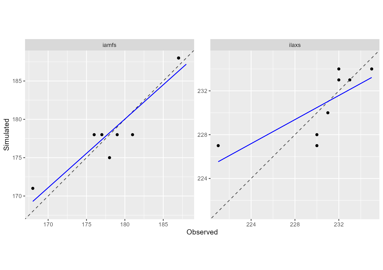

MSE and its components can be calcuted for each variable using the CroPlotR summary function:

summary(sim_after_optim$sim_list, obs = obs_list,
        stats = c("MSE", "Bias2", "SDSD", "LCS"))

## # A tibble: 2 × 7
##   group     situation      variable   MSE  Bias2   SDSD   LCS
##   <chr>     <chr>          <chr>    <dbl>  <dbl>  <dbl> <dbl>
## 1 Version_1 all_situations iamfs     4.38 0.0156 0.0637  4.92
## 2 Version_1 all_situations ilaxs     7    0.0625 1.14    6.78

Samuel Buis

2023-12-22