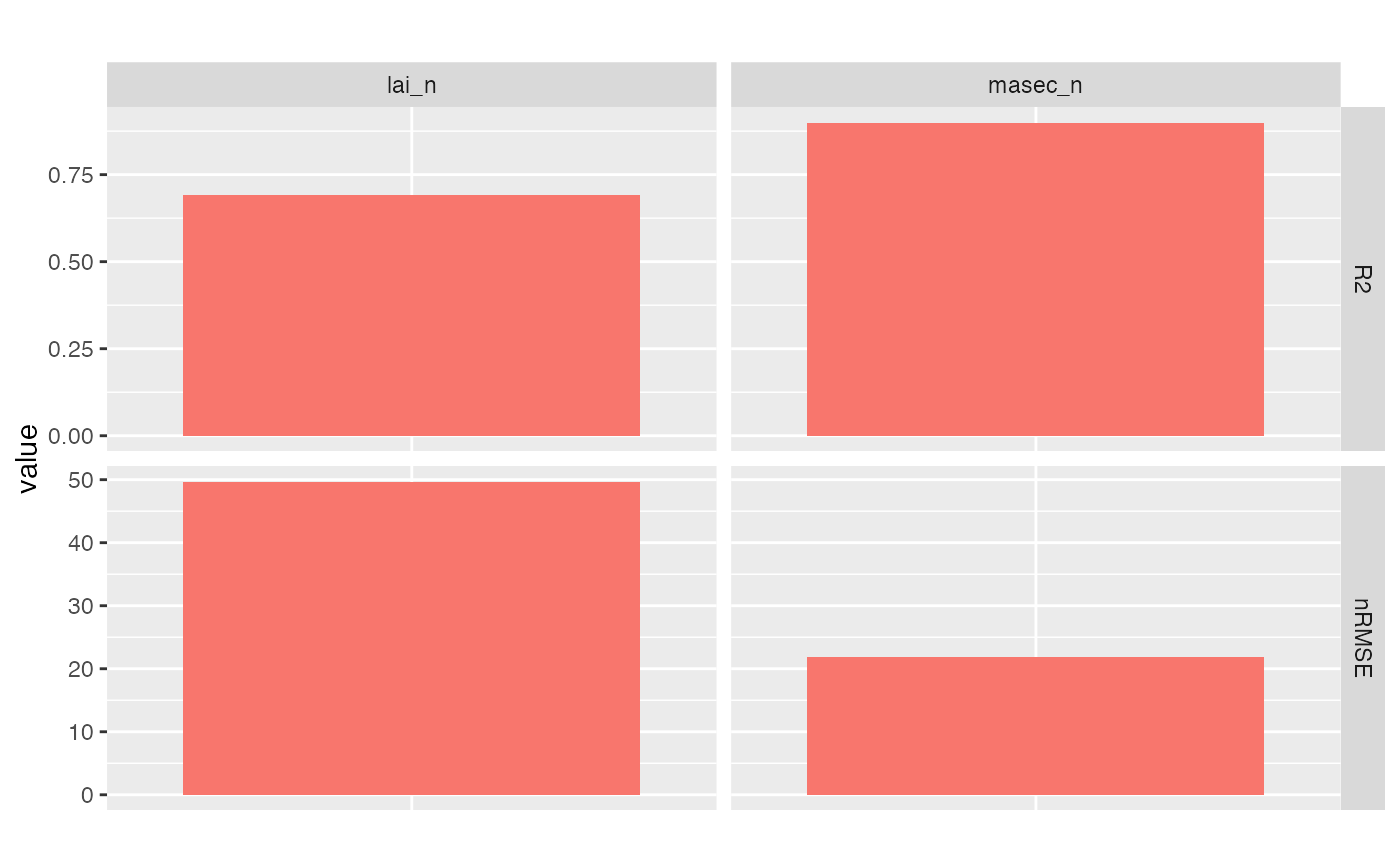
Plot statistics

Plot statistics

# S3 method for statistics
plot(
  x,
  xvar = c("group", "situation"),
  type = c("bar", "radar"),
  group_bar = c("rows", "stack", "dodge"),
  crit_radar = NULL,
  title = NULL,
  force = TRUE,
  verbose = TRUE,
  ...
)

Arguments

x

The output of summary.cropr_simulation()

xvar

The variable to use in x, either the group or the situation (the other is used for colouring)

type

The type of plot requested, either "bar" (bar plot) or "radar" (radar chart)

group_bar

Way to display the different statistical criteria when type= "bar". See details.

crit_radar

Statistical criterion chosen to be displayed on the radar chart.

title

The plot title

force

Continue if the plot is not possible ? E.g. no observations for scatter plots. If TRUE, return NULL, else return an error.

verbose

Boolean. Print information during execution.

...

Other arguments to pass (for backward compatibility only)

Value

Return a ggplot object with statistics

Details

The group_bar argument can be:

• "rows" (the default): One line of graphs per statistical criterion

• "stack": Bars of each statistical criterion stacked

• "dodge": Bars of each statistical criterion side by side

Examples

# Importing an example with three situations with observation:
workspace <- system.file(file.path("extdata", "stics_example_1"),
  package = "CroPlotR"
)
situations <- SticsRFiles::get_usms_list(
  usm_path =
    file.path(workspace, "usms.xml")
)
#> Warning: The `usm_path` argument of `get_usms_list()` is deprecated as of SticsRFiles
#> 1.0.0.
#> ℹ Please use the `file` argument instead.
sim <- SticsRFiles::get_sim(workspace = workspace, usm = situations)
#> mod_sSC_Pea_2005-2006_N0.sti
#> mod_sSC_Wheat_2005-2006_N0.sti
#> mod_spIC_Wheat_Pea_2005-2006_N0.stimod_saIC_Wheat_Pea_2005-2006_N0.sti
obs <- SticsRFiles::get_obs(workspace = workspace, usm = situations)
#> SC_Pea_2005-2006_N0.obs
#> SC_Wheat_2005-2006_N0.obs
#> IC_Wheat_Pea_2005-2006_N0p.obsIC_Wheat_Pea_2005-2006_N0a.obs

# R2 and nRMSE stats for the simulation:
stats <- summary(sim, obs = obs, stats = c("R2", "nRMSE"))
plot(stats)


# Change the group name:
stats <- summary("stics v9.0" = sim, obs = obs, stats = c("R2", "nRMSE"))
plot(stats)


# R2 and nRMSE stats for two groups of simulations:
summary(sim1 = sim, sim2 = sim, obs = obs, stats = c("R2", "nRMSE"))
#>   group      situation variable        R2    nRMSE
#> 1  sim1 all_situations    lai_n 0.6923882 49.68537
#> 2  sim1 all_situations  masec_n 0.8994510 21.83710
#> 3  sim2 all_situations    lai_n 0.6923882 49.68537
#> 4  sim2 all_situations  masec_n 0.8994510 21.83710